Lab 10

Localization and Bayes Filtering

For this lab I needed to download a fare amount of starting code and directories to get myself situated to do this lab. I used a Bayes Filter in the simulation to show accurate localization. I comapred this with no Bayes Filter to see the difference. To do this I had to implement a few helper functions to develop the Bayes filter algorithm.

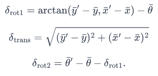
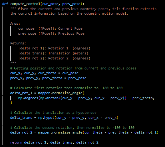
To implement compute control, I had it take the current and the previous pose and use their differene to determine the initial roation, translation, and final rotation.

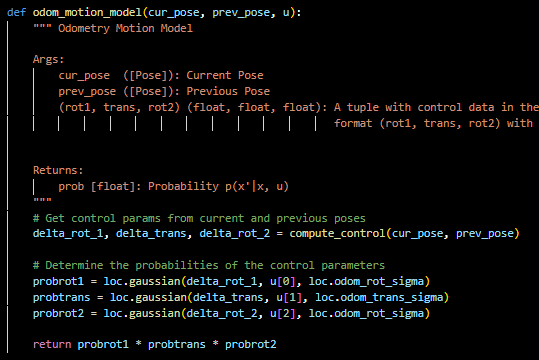
If we know our current and previous pose, this function extracts the odometry model parameters using compute_control(). Then it calculates the probabilities of these parameters as Gaussian distributions using the given standard deviations cetnered a control input u.

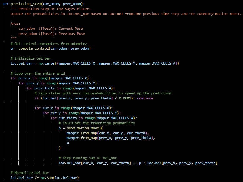
This function takes in the previous and current odometry state and extracts the odometry model parameters using compute control again. It iternates over the entire grid of cells from loc.bel.bar for the previous and current poses to construct a predicted belief. These probabilities are multiplied together and tallied then finally normalized as a distribution to sum to 1. I used Stephan's idea to ignore very small probabilites to speed up computation time.

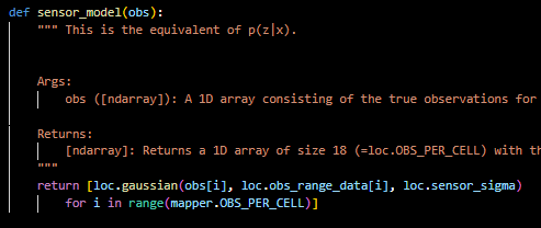
The sensor model uses the array of observations and calculates the probabilities of each occuring as a Guassian.

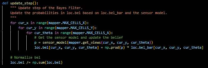
Finally this function iterates over the grid for the current state and using sensor model gets the sensor model data and then updates the belief bel. This updated belief is then normalized to sum to 1. This number is the robot's estimation of its position in the environment.

First Run

This is a video of the sim before bayes filter. As shown the odometry (red) goes everywhere.

Run 1 After Bayes Filter

After adding the Bayes filter the odometry model is a bit better. The Bayes probabilistic belief (blue) gives a good approximation of the robot's actual position. This is shown when the sensor is near the wall, the data is much better compared to when it is in the center of the map. Below is the raw data for 2 runs.

Step	Ground Truth State	Belief State	Belief Probability	Error
0	(0.316, -0.823, 170.275)	(0.293, -0.910, -200.000)	1.0	(-0.023, -0.087, 370.275)
1	(0.371, -0.995, 527.357)	(0.168, -0.909, -200.000)	1.0	(0.203, 0.086, 727.357)
2	(0.425, -1.166, 884.437)	(0.222, -1.088, -200.000)	1.0	(0.203, 0.086, 1084.437)
3	(0.446, -1.346, 1244.437)	(0.375, -1.338, -200.000)	1.0	(-0.071, -0.008, 1444.437)
4	(0.330, -1.494, 1590.379)	(0.214, -1.642, -200.000)	1.0	(-0.116, -0.148, 1790.379)
5	(0.279, -1.479, 1958.085)	(0.228, -1.494, -200.000)	0.9999999	(0.051, 0.015, 2158.085)
6	(0.279, -1.479, 1935.164)	(0.228, -1.479, -200.000)	1.0	(0.051, 0.000, 2135.164)
7	(0.279, -1.479, 1881.101)	(0.228, -1.596, -200.000)	1.0	(0.051, -0.117, 2081.101)
8	(0.177, -1.784, 1806.045)	(0.075, -2.089, -200.000)	1.0	(0.102, -0.305, 2006.045)
9	(0.177, -1.784, 1785.920)	(0.177, -2.089, -200.000)	1.0	(0.000, -0.305, 1985.920)
10	(0.177, -1.784, 1765.795)	(0.177, -2.089, -200.000)	1.0	(0.000, -0.305, 1965.795)
11	(0.177, -1.784, 1745.670)	(0.177, -2.089, -200.000)	1.0	(0.000, -0.305, 1945.670)
12	(0.177, -1.784, 1725.545)	(0.177, -1.479, -200.000)	1.0	(0.000, -0.305, 1925.545)
13	(0.177, -1.784, 1705.420)	(0.177, -1.479, -200.000)	1.0	(0.000, -0.305, 1905.420)
14	(0.177, -1.784, 1685.295)	(0.177, -1.479, -200.000)	1.0	(0.000, -0.305, 1885.295)
15	(-0.672, -0.090, 5939.583)	(-0.610, -0.305, -170.000)	0.9999998	(0.062, 0.215, 6109.583)

Run 2 After Bayes Filter

Step	Ground Truth State	Belief State	Belief Probability	Error
0	(0.287, -0.087, 320.561)	(0.305, 0.000, -50.000)	1.0	(-0.018, -0.087, 370.561)
1	(0.515, -0.523, 657.643)	(0.305, -0.610, -70.000)	1.0	(0.210, 0.087, 727.643)
2	(0.515, -0.523, 994.341)	(0.305, -0.610, -90.000)	1.0	(0.210, 0.087, 1084.341)
3	(0.545, -0.922, 1354.341)	(0.610, -0.914, -90.000)	1.0	(-0.064, -0.007, 1444.341)
4	(0.809, -1.064, 1799.806)	(0.610, 0.305, 90.000)	0.9999998	(0.200, -1.369, 1709.806)
5	(1.587, -0.909, 2208.143)	(1.524, -0.914, 50.000)	1.0	(0.063, 0.005, 2158.143)
6	(1.677, -0.526, 2596.797)	(1.829, -0.305, 90.000)	1.0	(-0.152, -0.221, 2506.797)
7	(1.760, -0.176, 2962.432)	(1.829, -0.305, 90.000)	1.0	(-0.069, 0.129, 2872.432)
8	(1.775, 0.316, 3345.069)	(1.829, 0.000, 90.000)	0.8765183	(-0.054, 0.316, 3255.069)
9	(1.787, 0.634, 3745.171)	(1.829, 0.914, 150.000)	1.0	(-0.042, -0.280, 3595.171)
10	(1.377, 0.920, 4116.442)	(1.524, 0.610, 150.000)	0.9999999	(-0.147, 0.310, 3966.442)
11	(0.495, 0.842, 4572.681)	(0.610, 0.914, -110.000)	1.0	(-0.114, -0.073, 4682.681)
12	(0.302, 0.221, 4977.763)	(0.305, 0.305, -70.000)	1.0	(-0.003, -0.084, 5047.763)
13	(0.050, -0.081, 5270.166)	(0.000, -0.305, -130.000)	1.0	(0.050, 0.224, 5400.166)
14	(-0.316, -0.225, 5607.147)	(-0.305, -0.305, -150.000)	1.0	(-0.011, 0.080, 5757.147)
15	(-0.709, -0.215, 5944.129)	(-0.610, -0.305, -170.000)	0.9998672	(-0.100, 0.090, 6114.129)